Coordinates

Example to familiarize with the coordinate system used by SRW.

Import PySRW module

import pysrw as srw

For this example, we use the same dipole as Simple dipole magnet

energy = 3.0    # GeV
rho = 7.047     # m
length = 1.384  # m
gap = 36e-3     # m

dipole = srw.magnets.Dipole(energy=energy, bendingR=rho,
                            coreL=length, edgeL=gap, centerCoord=[0,0,0])

We include the dipole in a MagnetsContainer(). We set lengthPadFraction = 2 to define an integration range twice as long as the total length of the dipole.

mag_container = srw.magnets.MagnetsContainer([dipole], lengthPadFraction=2.0)

The limits of the integration are therefore

zStart, zEnd, res = mag_container.getIntegrationParams()
print(f"Start: {zStart:.2f} - End: {zEnd:.2f}")

Start: -2.18 - End: 2.18

We use the default values for the ParticleBeam() initial position. This produces a beam that arrives at the centre of the dipole (z=0) at the rasverse position [0,0] and with angles [0,0].

beam = srw.emitters.ParticleBeam(energy, xPos=0, yPos=0, zPos=0,
                                 xAngle=0, yAngle=0)

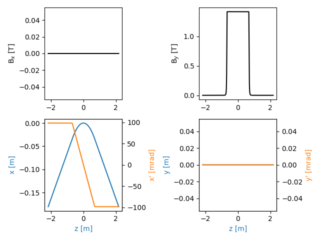
The particle trajectory can be computed and plotted using the function plotTrajectory(). We leave the default values of sStart and sEnd which are assumed as zStart and zEnd. Note that the positions along the curvilinear coordinate ‘s’ do not exactly correspond to the longitudinal positions ‘z’. However, when transverse deflections are small, the difference between ‘s’ and ‘z’ is almost negligible.

traj = srw.computeTrajectory(beam, mag_container)
srw.plotTrajectory(traj)

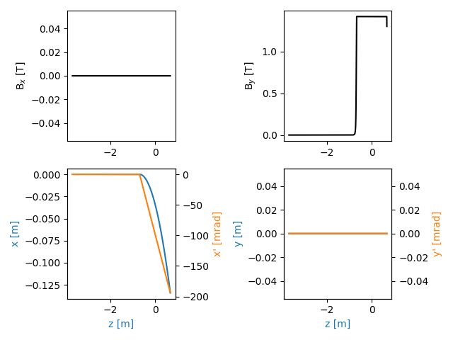
As a second case, we simulate a beam travelling along the axis [0,0] and then deflected by the dipole. We need to change the beam definition, setting the initial condition outside of the diple instead of at the dipole centre. Note that this does not affect the position of the dipole, which has still the centre at z = 0.

beam = srw.emitters.ParticleBeam(energy, xPos=0, yPos=0, zPos=-1.5,
                                 xAngle=0, yAngle=0)

To recompute the trajectory in this case, it is convenient to change the sStart and sEnd parameters. If we leave the default values, the trajectory computation ranges from sStart = -2.18 and sEnd = 2.18. Since the particle initial position is defined at z = -1.5, these limits do not cover the dipole extension as the trajectory starts more than 2 m before the magnet and ends approximately at z = 0.68, not entirely outside of the magnetic region.

traj = srw.computeTrajectory(beam, mag_container)
srw.plotTrajectory(traj)

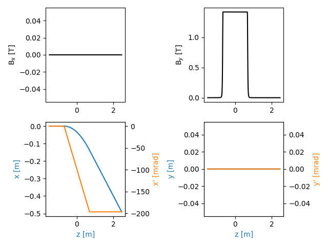
We can adjust the limits by choosing a sStart = 0 and sEnd = 4, so that the trajectory starts at the dipole entrance at sStart = -1.5, where the particle initial conditions were defined, and follows the beam for 4 m along the trajectory, thus well outside of the dipole.

traj = srw.computeTrajectory(beam, mag_container, sStart=0, sEnd=4)
srw.plotTrajectory(traj)

Estimated memory usage: 112 MB