Custom magnet

Example to show the simulation of a arbitrary magnetic field. A longitudinal gradient dipole from ESRF-EBS is implemented using the CustomMagnet.

Import modules required for simulations

import matplotlib.pyplot as plt
import numpy as np

import pysrw as srw

A longitudinal gradient dipole is a device where the magnetic field increases varies the propagation. The ideal device should feature a smooth variation of the magnetic field (continuous gradient dipole). This option is often not practical and, in real scenarios, it is more convenient to create a series of discrete magnetic steps.

energy = 6      # GeV
L_eff = 1.784   # total device length
B_start = 0.65  # the magnetic field at the magnet entrance
B_end = 0.17    # the magnetic field at the magnet exit
segments = 5    # number of steps of the magnetic field

A 3D map of the field components is required to define the device field. Since this particular case involve only a longitudinal change of the field, we can create field arrays with only one bin along the transverse direction. The longitudinal profile is a sequence of decreasing steps. We create a profile with 3 points per segment. This is not the final resolution of the field as SRW will interpolate the provided field map on the discretization step of the trajectory computation. Notice also that the actual extension of the magnetic field region is not the final one, as the field map will be adjusted to match the physical extension specified in the magnet definition

nx = 1
ny = 1
nz = segments * 3

B_profile = np.repeat(np.linspace(B_start, B_end, segments), nz // segments)

Bz = np.zeros((nx, ny, nz))
Bx = np.zeros((nx, ny, nz))
By = np.reshape(B_profile, (nx, ny, nz))

We create the magnetic object. The field map defined above is passed as a list with the three components. The argument ranges define the actual extension of the magnetic region. In this case, we will get a 1 m x 1m uniform field at each transverse plane and the field maps are adjusted to fit in a region of length L_eff. We also specify the strategy that is later used to interpolate the coarse mesh of the field map on the much finer discretization of the trajectory.

dipole = srw.magnets.CustomMagnet(magField=[Bx, By, Bz],
                                  ranges=[1,1,L_eff],
                                  interp="bilinear")

The device is wrapped as usual in a container and the beam is created with all zero initial conditions at the dipole entrance

mag_container = srw.magnets.MagnetsContainer([dipole])
beam = srw.emitters.ParticleBeam(energy, xPos=0, yPos=0, zPos=-1.5)

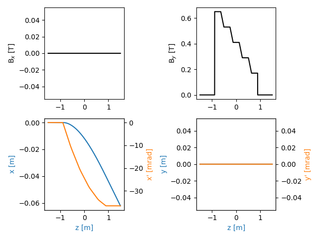
We finally compute the trajectory and plot a detailed view of the resulting custom field profile and trajectory. Note in particular how the user-defined field points are interpolated to create a continous field profile.

traj = srw.computeTrajectory(beam, mag_container, sStart=0, sEnd=3)
srw.plotTrajectory(traj)

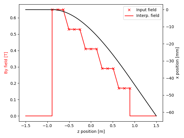
fig, ax_mag = plt.subplots()
ax_mag.plot(np.linspace(-.5, .5, nz) * L_eff, B_profile,
            linewidth=0, marker="x", color="red", label="Input field")
ax_mag.plot(traj["z"], traj["By"], color="red", label="Interp. field")
ax_trj = ax_mag.twinx()
ax_trj.plot(traj["z"], traj["x"] * 1e3, color="black")
ax_mag.set_xlabel("z position [m]")
ax_mag.set_ylabel("By field [T]", color="red")
ax_trj.set_ylabel("x position [mm]", color="black")
ax_mag.legend()
plt.tight_layout()
plt.show()

• 
• 

Estimated memory usage: 7 MB