Spectrum

Basic example of computation of synchrotron radiation spectrum.

Import modules required for simulations and for comparison with the theoretical distribution of dipole radiation.

import matplotlib.pyplot as plt
import numpy as np
from scipy.special import kv
from scipy.constants import e, epsilon_0, mu_0, c, pi, h

import pysrw as srw

We use the same source used for the simulation of the spatial distribution in the example Simple dipole magnet

energy = 3.0    # GeV
rho = 7.047     # m
length = 1.384  # m
gap = 36e-3     # m

dipole = srw.magnets.Dipole(energy=energy, bendingR=rho,
                            coreL=length, edgeL=gap)

mag_container = srw.magnets.MagnetsContainer([dipole])

beam = srw.emitters.ParticleBeam(energy, xPos=0, yPos=0, zPos=0)

The simulation of the radiation spectrum requires an Observer. The spectrum is computed at the observer centre, all other parameters can be ignored

observer = srw.wavefronts.Observer(centerCoord=[0, 0, 5])

The computation is performed with computeSpectrum(). In this example we request the computation of 1000 points between 0.01 and 10 nm. Keep in mind that the points are uniformely sampled along the photon energy axis. The points in the wavelength axis won’t be evenly distributed.

wfr = srw.computeSpectrum(particleBeam=beam,
                          magnetsContainer=mag_container,
                          observer=observer,
                          fromWavelength=.01, toWavelength=10, numPoints=1000,
                          srApprox="auto-wiggler")
spectrum = wfr.getSpectrumI()
srw.plotSpectrum(spectrum, axisScale=["log", "log"])

We compute the corresponding theoretical spectral distribution from the Schwinger model

r_p = observer.zPos
theta = 0
wl = wfr.wlax # nm
wl_c = dipole.getLambdaCritical() # nm
gamma = beam.nominalParticle.gamma

gt_sqr = (gamma * theta)**2
xi = wl_c/ (2 * wl) * (1 + gt_sqr)**(3/2)

e_theo_h = (-np.sqrt(3)*e*gamma) / ((2*pi)**(3/2) * epsilon_0 * c *r_p) *\
    (wl_c / (2 * wl)) * (1 + gt_sqr) * kv(2/3, xi)

e_theo_v = (1j*np.sqrt(3)*e*gamma) / ((2 * pi)**(3/2) * epsilon_0 * c *r_p) *\
    (wl_c / (2 * wl)) * (gamma * theta) * np.sqrt(1 + gt_sqr) * kv(1/3, xi)

int_theo = (4 * pi) / (mu_0 * c * wl*1e-9 * h * e) \
    * 1e-15 * (np.abs(e_theo_h)**2 + np.abs(e_theo_v)**2)

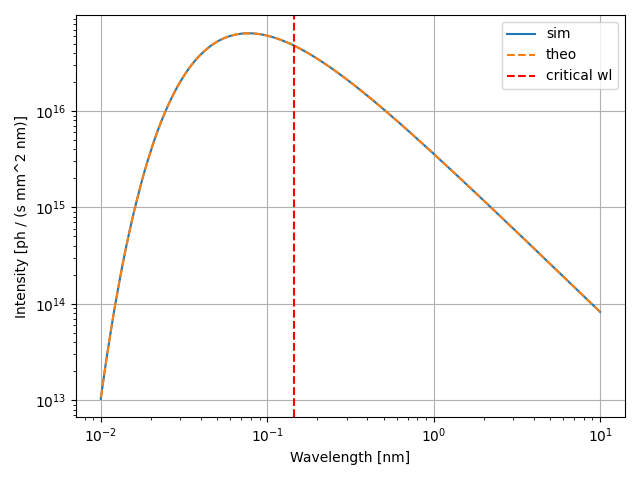
The final plot compares simulated and theoretical results. The curve exhibits the typical broadband emission of dipole radiation, with the critical wavelength dividing the spectrum in two regions of equal radiated power

fig, ax = plt.subplots()
ax.plot(wl, spectrum["data"], label="sim")
ax.plot(wl, int_theo, label="theo", linestyle="--")
ax.axvline(wl_c, label="critical wl", color="red", linestyle="--")
ax.set_xlabel("Wavelength [nm]")
ax.set_ylabel("Intensity [ph / (s mm^2 nm)]")
ax.set_xscale("log")
ax.set_yscale("log")
ax.grid()
ax.legend()
plt.tight_layout()
plt.show()

Estimated memory usage: 27 MB