Interferometer

A double slit interferometer with a point source. Multiprocess propagation is used to obtain the interferogram produced by different configurations of the optical system.

Import libraries required for simulation

from copy import deepcopy

import matplotlib.pyplot as plt
import numpy as np

import pysrw as srw

Create the wavefront arriving at the first plane of the optical system with parameters similar to Simple propagation

ptSrc = srw.emitters.PointSource()

observer = srw.wavefronts.Observer(centerCoord=[0, 0, .5],
                                   obsXextension=5e-3,
                                   obsYextension=5e-3,
                                   obsXres=1e-6,
                                   obsYres=1e-6)

wfr = srw.computePtSrcWfr(ptSrc, observer, wavelength=600)

w = 500e-6
d = 2e-3
f = 50e-3
s1 = observer.zPos
s2 = s1 * f / (s1 - f)

We use a rectangular aperture with an obstacle at the centre to create the two interferometer slits

optSystem = {
    "slitAp": {
        "type": "rectAp",
        "extension": [w, d + w],
        "centre": [0,0]
    },
    "slitOb": {
        "type": "rectOb",
        "extension": [2 * w, d - w],
        "centre": [0,0]
    },
    "lens": {
        "type": "lens",
        "f": f,
        "centre": [0,0]
    },
    "image": {
        "type": "drift",
        "length": s2,
        "resParam": {"hRangeChange": 1/20, "hResChange": 2.0,
                     "vRangeChange": 1/20, "vResChange": 2.0,
                     "hCentreChange": 0.0, "vCentreChange": 0.0}
    }
}

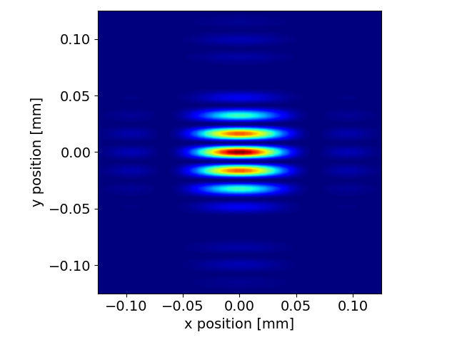
We proceed with a standard propagation to check that the parameters are good. As expected, the interferogram of the point emitter exhibits a unitary visibility and its envelope lies within the single slit diffraction pattern.

propData = srw.propagateWfr(wfr, optSystem, saveIntAt=["image"])
srw.plotI(propData["image"]["intensity"])

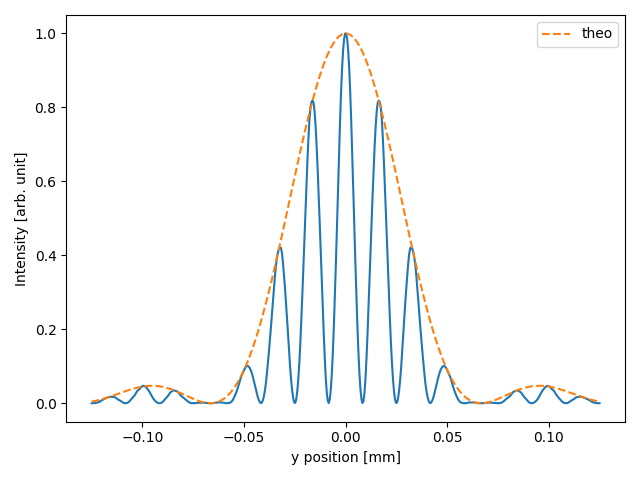
cuts = srw.extractCrossCuts(propData["image"]["intensity"])
yax = cuts["yax"]
int_srw = cuts["ydata"]
int_theo = np.sinc(w * yax / (s2 * wfr.wavelength*1e-9))**2

fig, ax = plt.subplots()
ax.plot(yax*1e3, int_srw / np.max(int_srw))
ax.plot(yax*1e3, int_theo, label="theo", linestyle="--")
ax.set_xlabel("y position [mm]")
ax.set_ylabel("Intensity [arb. unit]")
ax.legend()
plt.tight_layout()
plt.show()

• 
• 

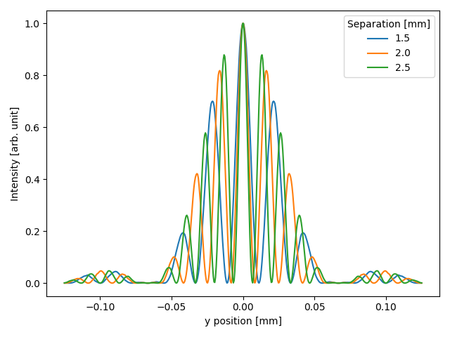
We can finally create a list of optical systems by changing the slit separation and observe the corresponding change in the fringe periodicity.

deltas = np.linspace(-.5, .5, 3) * 1e-3

optSystems = []
for delta in deltas:
    optSystemNew = deepcopy(optSystem)
    optSystemNew["slitAp"]["extension"][1] += delta
    optSystemNew["slitOb"]["extension"][1] += delta

    optSystems.append(optSystemNew)

propDatas = srw.propagateWfrMultiProcess(4, wfr, optSystems, saveIntAt=["image"])

fig, ax = plt.subplots()
for i, propData in enumerate(propDatas):
    cuts = srw.extractCrossCuts(propData["image"]["intensity"])
    yax = cuts["yax"]
    int_srw = cuts["ydata"]
    ax.plot(yax*1e3, int_srw / np.max(int_srw), label=f"{(d + deltas[i])*1e3}")
ax.set_xlabel("y position [mm]")
ax.set_ylabel("Intensity [arb. unit]")
ax.legend(title="Separation [mm]")
plt.tight_layout()
plt.show()

Estimated memory usage: 2288 MB