Gaussian beam

Basic example of computation of the field emitted by a coherent Gaussian beam.

Import required libraries

import matplotlib.pyplot as plt
import numpy as np

import pysrw as srw

Starts creating a coherent Gaussian beam with a waist of 20 um. We leave the default initial position and angle of the source (all zero)

sigma = 20e-6
gsnBeam = srw.emitters.GaussianBeam(xSigma=sigma, ySigma=sigma)

Create a 10 mm x 10 mm observation mesh, with a resolution of 100 um, placed 1 m downstream of the source

observer = srw.wavefronts.Observer(centerCoord=[0, 0, 1],
                                   obsXextension=10e-3,
                                   obsYextension=10e-3,
                                   obsXres=100e-6,
                                   obsYres=100e-6)

Compute the wavefront at the observation wavelength of 600 nm. The multiprocessing version is reported for comparison

wl = 600
wfr = srw.computeGsnBeamWfr(gsnBeam, observer, wavelength=wl)
wfr_mp = srw.computeGsnBeamWfrMultiProcess(4, gsnBeam, observer, wavelength=600)

Compute the corresponding optical intensity

intensity = wfr.getWfrI()
intensity_mp = wfr_mp.getWfrI()

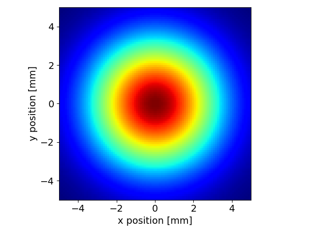
Plot the 2D intensity distribution

srw.plotI(intensity)
srw.plotI(intensity_mp)

• 
• 

Extract cross-cut using extractCrossCuts()

crosscuts = srw.extractCrossCuts(intensity)
xax = crosscuts["xax"]
xcut = crosscuts["xdata"]

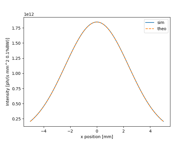
Compare the intensity profile with the theoretical distribution. For a Gaussian beam \(\sigma \cdot \sigma' = \lambda / 4 \pi\). We omit the spherical attenuation as it’s negligible with respect to the decay due to the finite divergence of the beam

sigma_p = wl*1e-9 / (4 * np.pi * sigma) #rad
xcut_theo = srw.gaussian1p(xax, sigma_p * observer.zPos)

Summary plot of the intensity cuts

fig, ax = plt.subplots()
ax.plot(xax * 1e3, xcut, label="sim")
ax.plot(xax * 1e3, np.max(xcut) * xcut_theo, linestyle="--", label="theo")
ax.set_xlabel("x position [mm]")
ax.set_ylabel("Intensity [ph/(s mm^2 0.1%BW)]")
ax.legend()
plt.show()

Estimated memory usage: 10 MB