Simple propagation

Basic example of physical optics propagation through a simple optical system consisting of a square aperture illuminated by a point source and focused by a thin lens.

Import libraries required for simulation

import matplotlib.pyplot as plt
import numpy as np

import pysrw as srw

Create the wavefront arriving at the first plane of the optical system as described in Point source. Check the section about propagation for some tips about the definition of the mesh parameters.

ptSrc = srw.emitters.PointSource()

observer = srw.wavefronts.Observer(centerCoord=[0, 0, .5],
                                   obsXextension=10e-3,
                                   obsYextension=10e-3,
                                   obsXres=1e-6,
                                   obsYres=1e-6)

wfr = srw.computePtSrcWfr(ptSrc, observer, wavelength=600)

We use a basic optical system consisting of a square aperture and a thin lens and we observe the intensity at the image plane of the lens.

w = 500e-6
f = 50e-3
s1 = observer.zPos
s2 = s1 * f / (s1 - f)

The optical system is created as a dictionary representing the three optical elements. Note that “aperture”, “lens” and “image” are arbitrary names. The nature of each optical element is defined by its “type” key

optSystem = {
    "aperture": {
        "type": "rectAp",
        "extension": [w, w],
        "centre": [0,0]
    },
    "lens": {
        "type": "lens",
        "f": f,
        "centre": [0,0]
    },
    "image": {
        "type": "drift",
        "length": s2
    }
}

The propagation is performed using the propagateWfr() function. Since we leave all optional arguments to their default values, the sequence [“lens”, “drift”] will be grouped, the intensity stored on all planes and the wavefront only at the last “image” plane.

propData = srw.propagateWfr(wfr, optSystem)

We plot the resulting intensity distribution at the “aperture” and “image” planes

srw.plotI(propData["aperture"]["intensity"])
srw.plotI(propData["image"]["intensity"])

• 
• 

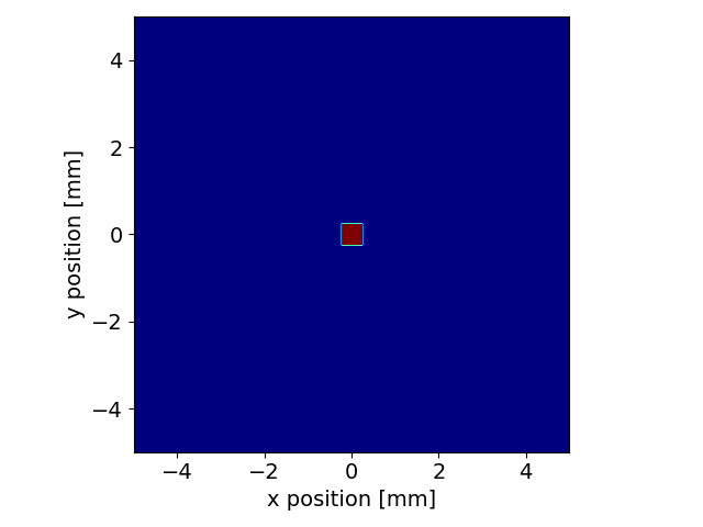
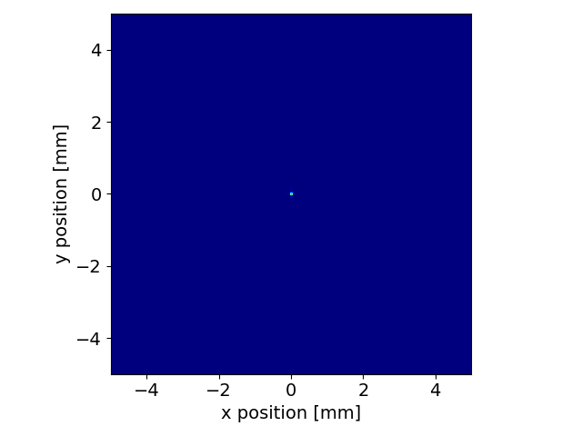
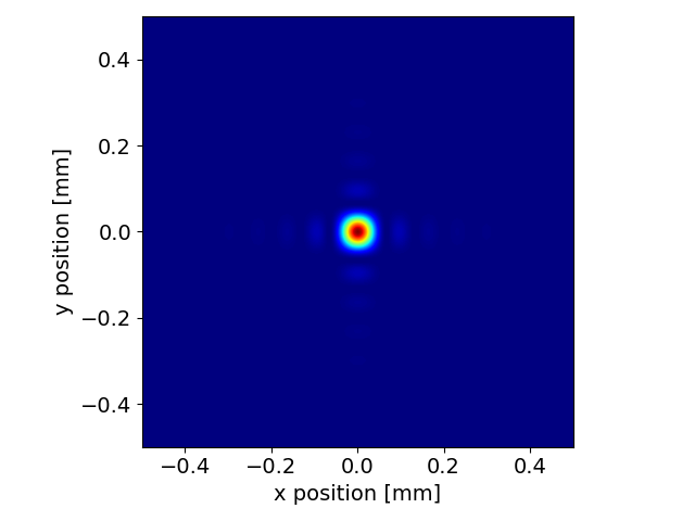
As expected, the final spot is much smaller with respect to the simulated wavefront. The extended wavefront is necessary at the entrance of the optical system, to leave enough margin around the aperture. However, the extension can be significantly reduced at the image plane, as the light is focused by the lens. This can be achieved by adding some resize parameters to reduce by a factor 10 the extension and increase by a factor 2 the resolution to obtain a smoother profile

optSystem["image"]["resParam"] = {"hRangeChange": 1/10, "hResChange": 2.0,
                                  "vRangeChange": 1/10, "vResChange": 2.0,
                                  "hCentreChange": 0.0, "vCentreChange": 0.0}

The computation is then repeated. To save time and memory, we store the intensity only at the final “image” plane

propData = srw.propagateWfr(wfr, optSystem, saveIntAt=["image"])
srw.plotI(propData["image"]["intensity"])

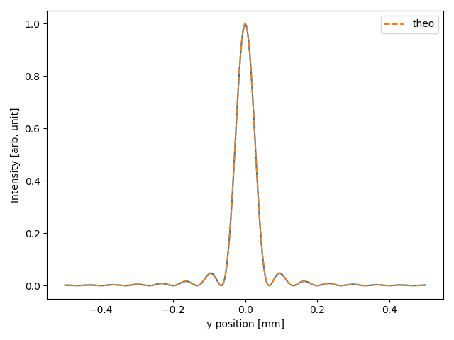
We can finally extract a profile and compare the simulated pattern with the sinc profile of the diffraction from a rectangular aperture

cuts = srw.extractCrossCuts(propData["image"]["intensity"])
yax = cuts["yax"]
int_srw = cuts["ydata"]
int_theo = np.sinc(w * yax / (s2 * wfr.wavelength*1e-9))**2

fig, ax = plt.subplots()
ax.plot(yax*1e3, int_srw / np.max(int_srw))
ax.plot(yax*1e3, int_theo, label="theo", linestyle="--")
ax.set_xlabel("y position [mm]")
ax.set_ylabel("Intensity [arb. unit]")
ax.legend()
plt.show()
plt.tight_layout()

Estimated memory usage: 4596 MB