LHC source

Evolution of the wavefront emitted by the LHC source during the energy ramp. This examples shows how to setup a simulation with protons and to use one of the predefined magnetic provided by the PySRW module.

We import the usual packages, along with the animation submodule of matploitlib needed to create the sequence of the wavefront evolution.

import matplotlib.pyplot as plt
import numpy as np
import matplotlib.animation as animation

import pysrw as srw

The PySRW library is initialized with ‘proton’.

srw.CONFIG.initParticleType("proton")

The magnetic container can be directly created calling the function predefinedLHCsource(), passing the beam energy. In order to include all devices of the LHC source, we leave the sourceFlag parameter to its default value ‘D3undD3’. Note that, by convention, the origin of the longitudinal coordinate (z=0) is set at the undulator centre. We initialize the beam at z=-3, leaving both transverse positions and angles to zero.

energy = 450    # GeV

mag_container = srw.magnets.predefinedLHCsource(energy)
beam = srw.emitters.ParticleBeam(energy, xPos=0, yPos=0, zPos=-3)

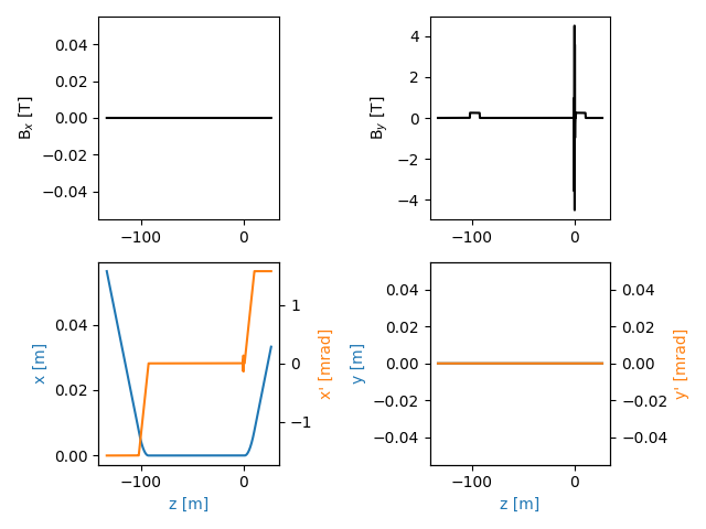
The trajectory is simulated to check the good instantiaiton of the objects. We track the particle between s=-130 and s=30, to include both D3 dipoles. As expected from the choice of the beam initial conditions, the beam travels along the longitudinal axis in the straight section between the dipoles.

traj = srw.computeTrajectory(beam, mag_container, sStart=-130, sEnd=30)
srw.plotTrajectory(traj)

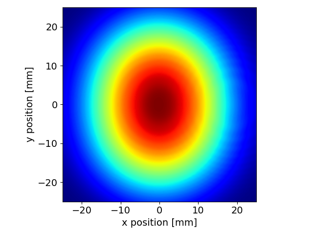
We simulate the distribution of the emitted wavefront. Since we will not propagate it through an optical system, we can define a rather coarse observation mesh to make the simulation faster.

wl = 560        # nm
observer = srw.wavefronts.Observer(centerCoord=[0, 0, 27.24],
                                   obsXextension=50e-3,
                                   obsYextension=50e-3,
                                   obsXres=200e-6,
                                   obsYres=200e-6)


wfr = srw.computeSrWfrMultiProcess(numCores=4,
                        particleBeam=beam, magnetsContainer=mag_container,
                        observer=observer, wavelength=wl)
intensity = wfr.getWfrI()
srw.plotI(intensity)

Finally, we can iterate the above caluclation changing the beam energy and following the evolution of the spatial intensity as a function of the beam energy (and at the fixed wavelength of 560 nm). This simulation clearly shows the undulator radiation that dominates the emission at injection. As the energy increases, the visible undulator radiation drifts to larger polar angles outside of our mesh. Above 1 TeV, dipole radiation appears first in form of edge radiation and later as core radiation. Circular fringes due to the interference between the two D3s are also clearly visible.

energies = [450, 550, 800, 1600, 3300, 6800]

frames = []
fig, ax = plt.subplots()
ax.set_xlabel("x position [mm]")
ax.set_xlabel("y position [mm]")
extent = np.array([intensity["xax"][0], intensity["xax"][-1],
                   intensity["yax"][0], intensity["xax"][-1]]) * 1e3

for energy in energies:

    mag_container = srw.magnets.predefinedLHCsource(energy)
    beam = srw.emitters.ParticleBeam(energy, xPos=0, yPos=0, zPos=-3)

    wfr = srw.computeSrWfrMultiProcess(numCores=4,
                        particleBeam=beam, magnetsContainer=mag_container,
                        observer=observer, wavelength=wl)
    intensity = wfr.getWfrI()

    frame = ax.imshow(intensity["data"], cmap="jet", extent=extent)
    annotation = ax.annotate(f"Energy: {energy:.0f} GeV",
                             (.05,.95), xycoords="axes fraction",
                             color="white", fontsize=12)
    frames.append([frame, annotation])

anim = animation.ArtistAnimation(fig, frames,
                                 interval=500, blit=True, repeat_delay=1000)

Once Loop Reflect

Estimated memory usage: 528 MB