Helical undulator

This example shows how to combine two planar undulators to create a helical undulator. The parameters of the single device are similar to the ones already used for the Simple planar undulator example.

Import modules required for simulations

import matplotlib.pyplot as plt
import numpy as np

import pysrw as srw

A helical undulator is the superposition of two perpendicular planar undulators with a phase delay of \(\phi\) which produces a rotation of the magnetic field along the device. In this example, the transverse field components are a shorter version of the undulator of NCD beamline at the ALBA light source

energy = 3.0        # GeV
lambda_u = 0.0216   # m
N_u = 5             # instead of 92 to better render the particle trajectory
B_0 = 0.75          # T

The magnet is created with the default SRW model for planar undulators

phi = np.pi/2
und_h = srw.magnets.UndulatorPlanar(energy=energy, undPlane="h",
                                    undPeriod=lambda_u, numPer=N_u,
                                    magField=B_0)
und_v = srw.magnets.UndulatorPlanar(energy=energy, undPlane="v",
                                    undPeriod=lambda_u, numPer=N_u,
                                    magField=B_0, initialPhase=phi)

We embed the two components in the a magnetic container. Note that it doesn’t matter if the two devices overlap. The total field is going to be a superposition of all component

mag_container = srw.magnets.MagnetsContainer([und_h, und_v],
                                             lengthPadFraction=2)

The last input for the simulation is the emitter, instance of ParticleBeam()

beam = srw.emitters.ParticleBeam(energy, xPos=0, yPos=0, zPos=-0.1)

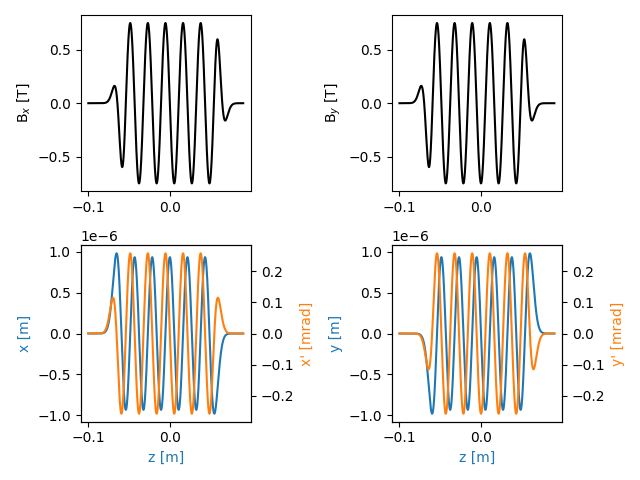
Before computing the wavefront, it is a good practice to obtain and plot the particle trajectory and check that the simulation objects properly defined

traj = srw.computeTrajectory(beam, mag_container, sStart=0, sEnd=0.2)
srw.plotTrajectory(traj)

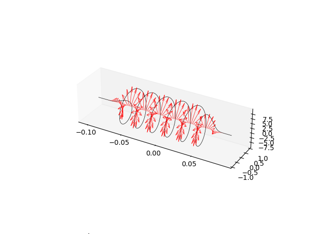
We can plot the trajectory and magnetic field in a 3D plot to better see the particle spiral and the field rotation along the device.

skip = 50 # sample few points for better readibility
z = traj["z"][::skip]
Bx = traj["Bx"][::skip] / np.max(traj["Bx"][::skip]) * np.max(traj["x"][::skip])
By = traj["By"][::skip] / np.max(traj["By"][::skip]) * np.max(traj["y"][::skip])
zeros = np.zeros(len(z))

fig = plt.figure()
ax = fig.add_subplot(111, projection="3d")
ax.set_box_aspect((4, 1, 1))
ax.plot(traj["z"], traj["x"], traj["y"], linewidth=0.5, color="black")
ax.quiver(z, zeros, zeros, zeros, Bx, By, linewidth=0.5, color="red")
ax.grid(False)
plt.show()

Create a 5 mm x 5 mm observation mesh, with a resolution of 10 um, placed 10 m downstream of the source

observer = srw.wavefronts.Observer(centerCoord=[0, 0, 10],
                                   obsXextension=5e-3,
                                   obsYextension=5e-3,
                                   obsXres=10e-6,
                                   obsYres=10e-6)

The simulation of the wavefront is done in the same way as the simple undulator case. The expression for the foundamental harmonic is slightly different

gamma = beam.nominalParticle.gamma
K = und_h.getK()
wl = lambda_u / (2 * gamma**2) * (1 + K**2) * 1e9

because the motion along the two transverse direction implies a term \(K^2\) instead of \(K^2/2\) derived for the planar undulator.

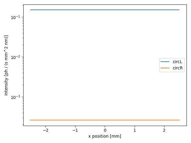
We finally simulate the wavefront and plot the intensity. The peculiarity of the helical undulator is the strong circluar polarization of the emitted light, whereas the plane undulator radiation is essentially linearly polarized

wfr = srw.computeSrWfrMultiProcess(4, particleBeam=beam,
                                   magnetsContainer=mag_container,
                                   observer=observer, wavelength=wl)
intensity_left = wfr.getWfrI(pol="circL")
intensity_right = wfr.getWfrI(pol="circR")

We can prove this by plotting a the central intensity crosscut for the circular-left and circular-right components. The sense of rotation of the circular polarization can be adjusted with the phase between the two components of the magnetic field. The phase \(\pi /2\) produces an essentially circular-left polarization, which can be transformed to circular-right by setting an opposite phase of \(-\pi /2\)

fig, ax = plt.subplots()
for pol in ["circL", "circR"]:
    intensity = wfr.getWfrI(pol=pol)
    cuts = srw.extractCrossCuts(intensity)
    ax.plot(cuts["xax"]*1e3, cuts["xdata"], label=pol)
ax.set_xlabel("x position [mm]")
ax.set_ylabel("Intensity [ph / (s mm^2 nm)]")
ax.set_yscale("log")
ax.legend()
plt.tight_layout()
plt.show()

Estimated memory usage: 11 MB