Point source

Basic example of computation of the field emitted by an isotropic point source.

Import required libraries

import matplotlib.pyplot as plt
import numpy as np

import pysrw as srw

Ccreate the point emitter radiating 1 ph/(s mm^2)

ptSrc = srw.emitters.PointSource(flux=1)

Create a 10 mm x 10 mm observation mesh, with a resolution of 10 um, placed 10 cm downstream of the source

observer = srw.wavefronts.Observer(centerCoord=[0, 0, .1],
                                   obsXextension=10e-3,
                                   obsYextension=10e-3,
                                   obsXres=10e-6,
                                   obsYres=10e-6)

Compute the wavefront at the observation wavelength of 600 nm. The multiprocessing version is reported for comparison

wfr = srw.computePtSrcWfr(ptSrc, observer, wavelength=600)
wfr_mp = srw.computePtSrcWfrMultiProcess(4, ptSrc, observer, wavelength=600)

Compute the corresponding optical intensity

intensity = wfr.getWfrI()
intensity_mp = wfr_mp.getWfrI()

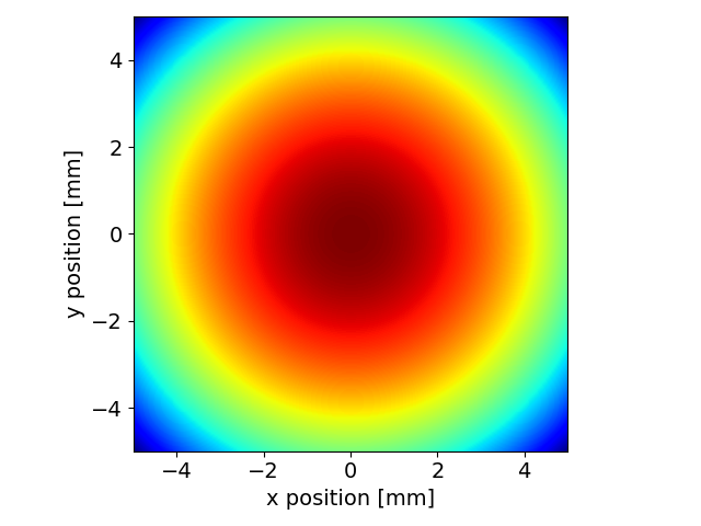
Plot the 2D intensity distribution

srw.plotI(intensity)
srw.plotI(intensity_mp)

• 
• 

Extract cross-cut using extractCrossCuts()

crosscuts = srw.extractCrossCuts(intensity)
xax = crosscuts["xax"]
xcut = crosscuts["xdata"]

Compare with the intensity decay due to spherical attenuation

theta = np.arctan(xax / observer.zPos)
xcut_theo = 1/(4 * np.pi * observer.zPos**2) * np.cos(theta)**3 * 1e-6 # ph / (s mm^2)

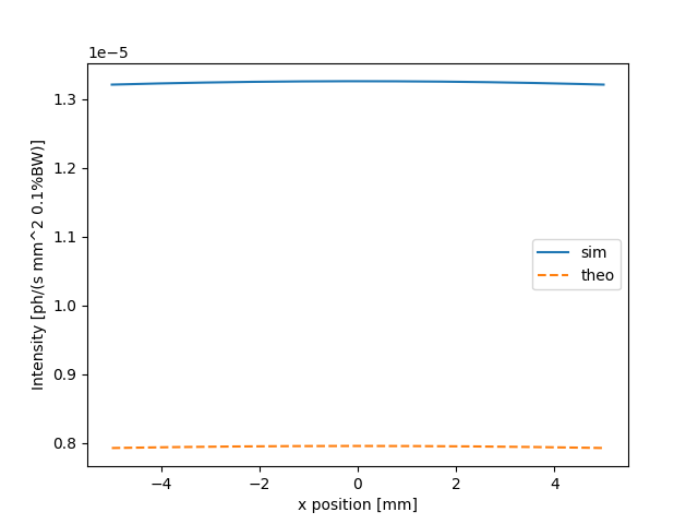
Plot the resulting cuts

fig, ax = plt.subplots()
ax.plot(xax * 1e3, xcut, label="sim")
ax.plot(xax * 1e3, xcut_theo, linestyle="--", label="theo")
ax.set_xlabel("x position [mm]")
ax.set_ylabel("Intensity [ph/(s mm^2 0.1%BW)]")
ax.legend()
plt.show()

Estimated memory usage: 80 MB