Transmission element

Example to demonstrate the flexibility of SRW propagation with the definition of a custom transmission element, given its transmissivity and phase delay. This specific example involves the creation of a four-quadrant phase mask, a special type of waveplate that delays by \(\pi\) two half planes of the wavefront.

Import libraries required for simulation

import matplotlib.pyplot as plt
import numpy as np

import pysrw as srw

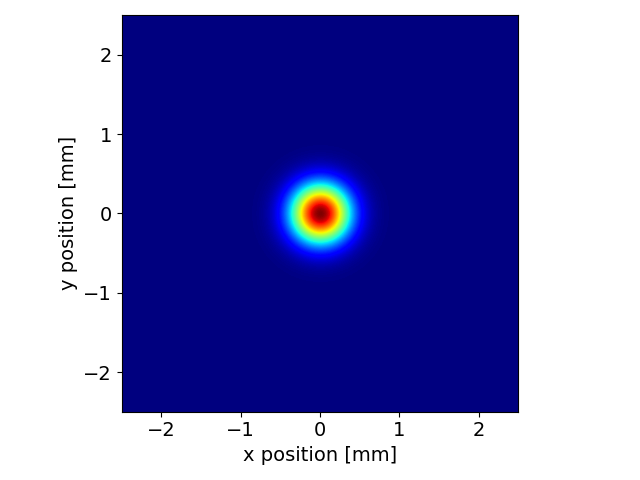
Create the wavefront arriving at the first plane of the optical system with parameters similar to Simple propagation. For this example we use a Gaussian beam instead of the point source.

ptSrc = srw.emitters.GaussianBeam()

observer = srw.wavefronts.Observer(centerCoord=[0, 0, .5],
                                   obsXextension=5e-3,
                                   obsYextension=5e-3,
                                   obsXres=1e-6,
                                   obsYres=1e-6)

wfr = srw.computeGsnBeamWfr(ptSrc, observer, wavelength=600)
srw.plotI(wfr.getWfrI())

The optical system consists of the phase mask with its aperture, a lens and a drift to focus the light.

w = 1e-3
f = 50e-3
s1 = observer.zPos
s2 = s1 * f / (s1 - f)

The transmission element is created passing a matrix for the optical path difference (in nm) amd one for the amplitude. Note that the initial extension

of this matrices is not important, because the actual extension of the

optical element will be given by its ‘extension’ value.

xx, yy = np.meshgrid(np.linspace(-1, 1, 1001), np.linspace(-1, 1, 1001))

opd = np.where(xx * yy > 0, wfr.wavelength / 2, 0)
amp = np.ones(np.shape(xx))

The mask is placed in the optical system dictionary as a standard optical element, specifying the ‘transmission’ type.

optSystem = {
    "aperture": {
        "type": "rectAp",
        "extension": [w, w],
        "centre": [0,0]
    },
    "mask": {
        "type": "transmission",
        "extension": [w, w],
        "centre": [0,0],
        "opd": opd,
        "amp": amp
    },
    "lens": {
        "type": "lens",
        "f": f,
        "centre": [0,0]
    },
    "image": {
        "type": "drift",
        "length": s2,
        "resParam": {"hRangeChange": 1/10, "hResChange": 1.0,
                     "vRangeChange": 1/10, "vResChange": 1.0,
                     "hCentreChange": 0.0, "vCentreChange": 0.0}
    },
}

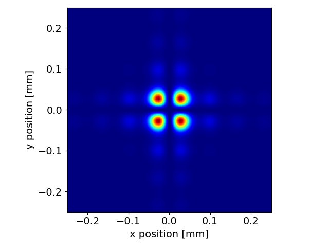
We finally propagate the field and plot the intensity at the image plane. One can clearly observe that the intensity has two nodes along the vertical and horizontal axis, corresponding to the region of destructive interference created by the phase mask.

propData = srw.propagateWfr(wfr, optSystem, saveWfrAt=optSystem.keys())
srw.plotI(propData["image"]["intensity"])

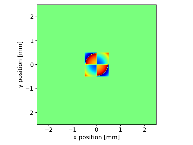
It is also possible to extract and plot the wavefront phase downstream of the mask. The \(\pi\) phase jump is indeed present, on top of the circular modulation of the phase due to the spherical wavefront.

phase = propData["mask"]["wfr"].getWfrPhase()
srw.plotI(phase)