Simple dipole magnet

Basic example of computation of the field emitted by an electron beam deflected by a simple dipole magnet.

Import modules required for simulations and for comparison with the theoretical distribution of dipole radiation.

import matplotlib.pyplot as plt
import numpy as np
from scipy.special import kv
from scipy.constants import e, epsilon_0, mu_0, c, pi, h

import pysrw as srw

We take as example the parameters of a typical bending magnet of a third-generation light source (ALBA-Spain)

energy = 3.0    # GeV
rho = 7.047     # m
length = 1.384  # m
gap = 36e-3     # m

which produce a particle deflection of

delta = 2 * np.arcsin(length / 2 / rho)
print(f"Deflection angle: {delta*1e3:.2f} mrad")

Deflection angle: 196.71 mrad

The magnet is created with the default SRW model for dipoles

dipole = srw.magnets.Dipole(energy=energy, bendingR=rho,
                            coreL=length, edgeL=gap)

This dipole emits a broad band radiation with a critical wavelength

wl_c = dipole.getLambdaCritical()
print(f"Critical wavelength: {wl_c:.2f} nm")

Critical wavelength: 0.15 nm

The magnetic element must be included in a magnetic container. In this simple example, the dipole is the only device and the limits for the numerical integration as left as default.

mag_container = srw.magnets.MagnetsContainer([dipole])

The last input for the simulation is the emitter, instance of ParticleBeam()

beam = srw.emitters.ParticleBeam(energy, xPos=0, yPos=0, zPos=0)

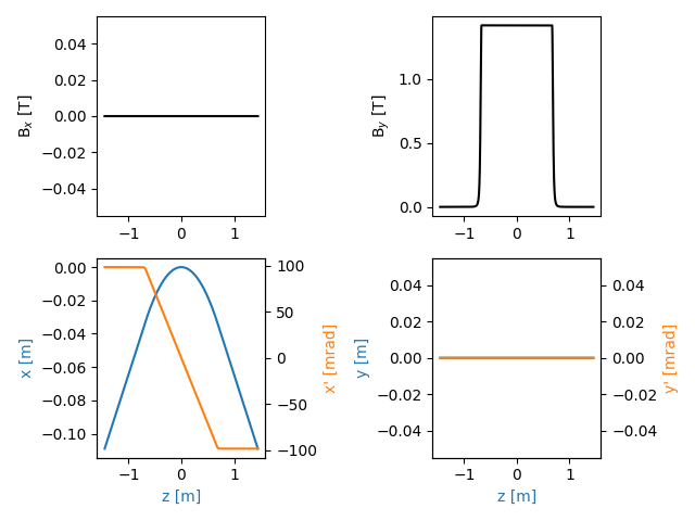
Before computing the wavefront, it is a good practice to obtain and plot the particle trajectory and check that the simulation objects properly defined

traj = srw.computeTrajectory(beam, mag_container)
srw.plotTrajectory(traj)

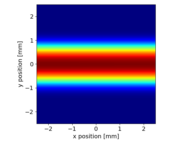
Create a 10 mm x 10 mm observation mesh, with a resolution of 100 um, placed 1 m downstream of the source

observer = srw.wavefronts.Observer(centerCoord=[0, 0, 5],
                                   obsXextension=5e-3,
                                   obsYextension=5e-3,
                                   obsXres=200e-6,
                                   obsYres=20e-6)

We can finally simulate the wavefront and derive the optical intensity, for example at the critical wavelength. Note that, dealing with a dipole, we use the “auto-wigggler” value for SR_APPROX()

wl = wl_c
wfr = srw.computeSrWfrMultiProcess(4, particleBeam=beam,
                                   magnetsContainer=mag_container,
                                   observer=observer, wavelength=wl,
                                   srApprox="auto-wiggler")
intensity = wfr.getWfrI()
srw.plotI(intensity)

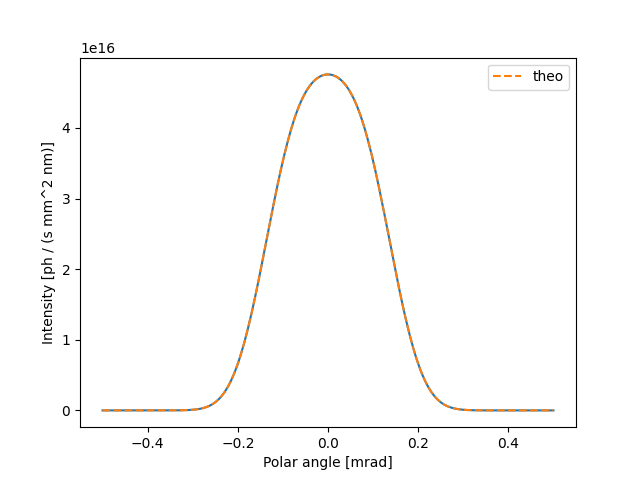
The distribution of SR emitted by a particle in a uniform field has an analytical expression. Let’s compare it to the simulation result. We extract a vertical slice from the simulation radiation

cuts = srw.extractCrossCuts(intensity)
yax = cuts["yax"]

and we derive the theoretical expression (Schwinger distributions)

r_p = observer.zPos
theta = np.arctan(yax / r_p)
gamma = beam.nominalParticle.gamma

gt_sqr = (gamma * theta)**2
xi = wl_c/ (2 * wl) * (1 + gt_sqr)**(3/2)

e_theo_h = (-np.sqrt(3)*e*gamma) / ((2*pi)**(3/2) * epsilon_0 * c *r_p) *\
    (wl_c / (2 * wl)) * (1 + gt_sqr) * kv(2/3, xi)

e_theo_v = (1j*np.sqrt(3)*e*gamma) / ((2 * pi)**(3/2) * epsilon_0 * c *r_p) *\
    (wl_c / (2 * wl)) * (gamma * theta) * np.sqrt(1 + gt_sqr) * kv(1/3, xi)

int_theo = (4 * pi) / (mu_0 * c * wl*1e-9 * h * e) \
    * 1e-15 * (np.abs(e_theo_h)**2 + np.abs(e_theo_v)**2)

Simulated and theoretical distributions are finally plotted

fig, ax = plt.subplots()
ax.plot(theta*1e3, cuts["ydata"])
ax.plot(theta*1e3, int_theo, label="theo", linestyle="--")
ax.set_xlabel("Polar angle [mrad]")
ax.set_ylabel("Intensity [ph / (s mm^2 nm)]")
ax.legend()
plt.show()

Estimated memory usage: 33 MB